
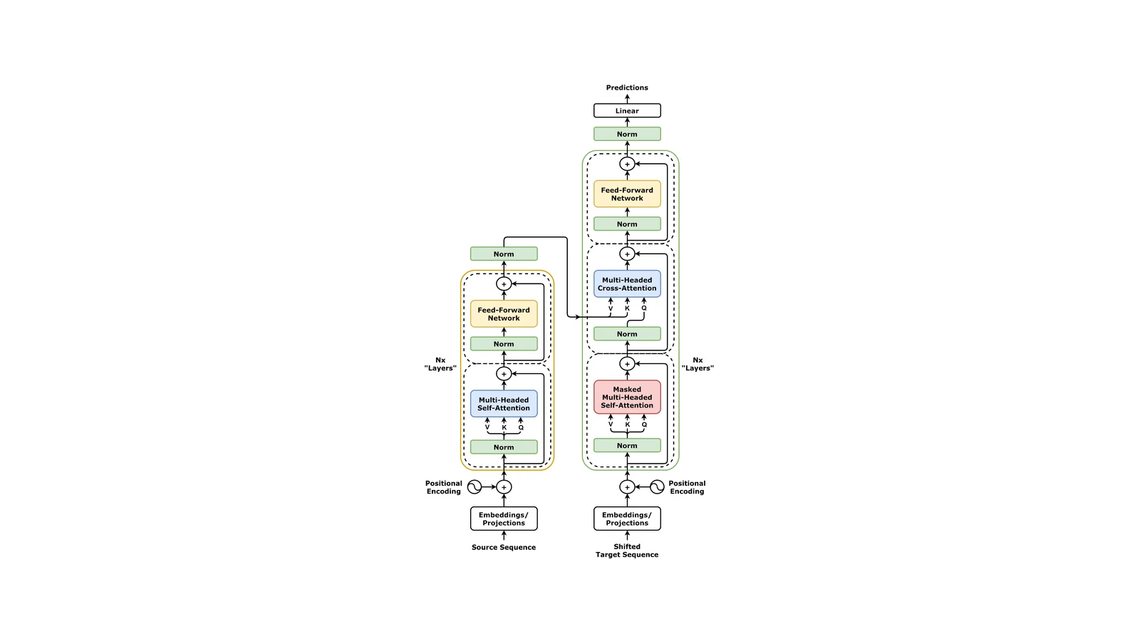
How Transformers Actually Work: A Walkthrough Without the Hand-Waving
Most explanations of transformers show you the diagram from the original paper and then describe the boxes. That tells you the architecture but not the mechanism, and it leaves the central question unanswered: why does attention work?
This walkthrough goes the other way. We will follow one token through the stack and watch what happens to it. By the end you should be able to explain why attention is the right primitive, what the feed-forward layers are actually for, and why the residual connections are more important than they look.
The problem transformers solved
Before 2017, sequence models were recurrent. You processed one token, updated a hidden state, processed the next. The hidden state carried everything you knew so far.
Two problems, both fatal at scale.
It cannot parallelise. Token five needs the state after token four. Training is inherently sequential, which wastes the one thing GPUs are good at.
Information decays. Everything about token one has to survive being repeatedly mixed and overwritten through hundreds of updates before it reaches token five hundred. LSTMs and GRUs made this better. They did not make it good.
The transformer's answer was to throw out recurrence entirely. Every token gets to look at every other token directly, in one step, in parallel. Position five reads position one as easily as position four.
The cost is that you no longer get order for free. A recurrent network knows about sequence because it is a sequence. A transformer sees a bag of vectors and has to be told about position explicitly. We will come back to that.
Step one: tokens become vectors
Text arrives as a string. The first job is turning it into numbers.
A tokenizer splits text into subword units: chunks that fall between characters and whole words. Common words are single tokens; rare ones split into pieces. "unhappiness" might become ["un", "happiness"] or ["unh", "appiness"], depending on the vocabulary.
Each token maps to an integer id, and each id indexes a row in an embedding matrix:
# vocab_size = 50000, d_model = 768
embedding = nn.Embedding(50000, 768)

token_ids = [1045, 2003, 1037]      # "this is a"
x = embedding(token_ids)             # shape: (3, 768)
Every token is now a 768-dimensional vector. These vectors are learned: nothing about the initial values means anything, and training pushes them into an arrangement where geometric relationships encode semantic ones. Similar words end up near each other because that makes the prediction task easier.
Step two: telling the model about position
Our three vectors carry no order information. Shuffle them and the model cannot tell.
Two families of solutions.
Absolute positional encoding adds a position-dependent vector to each embedding. The original paper used fixed sinusoids of different frequencies. Position 0 gets one pattern, position 1 another, and the pattern varies smoothly enough that the model can learn to read relative offsets from it. Later models learned the position vectors instead of fixing them.
Rotary positional embeddings (RoPE) are what nearly every current model uses, and they work differently. Rather than adding to the embedding, RoPE rotates the query and key vectors by an angle proportional to position, inside the attention computation.
The elegance is that the dot product between a query at position m and a key at position n ends up depending only on m − n. Relative position falls out of the geometry instead of being learned. This is why RoPE extrapolates to longer sequences better than absolute encodings, and it is a large part of how modern long-context models are possible.
Step three: attention, from first principles
Here is the core idea, and it is better built up than stated.
Each token needs to gather information from other tokens. But not uniformly. In "the animal did not cross the street because it was too tired," the token it needs animal specifically, and mostly needs to ignore street.
So each token needs to (a) express what it is looking for, (b) let other tokens express what they offer, and (c) match the two. That is exactly three projections:
- Query (Q): what this token is looking for.
- Key (K): what this token can be matched against.
- Value (V): what this token will contribute if matched.
The database analogy is genuinely helpful: a query is matched against keys, and you retrieve values. The difference is that instead of one exact match, you get a weighted blend of all values, weighted by how well each key matched.
Q = x @ W_q     # (seq, d_k)
K = x @ W_k     # (seq, d_k)
V = x @ W_v     # (seq, d_v)

scores  = Q @ K.T / sqrt(d_k)     # (seq, seq)
weights = softmax(scores, dim=-1)
output  = weights @ V             # (seq, d_v)
Four lines. Walk through them:
Q @ K.T computes every query against every key. Entry [i][j] is how much token i cares about token j. This matrix is the whole game: a learned, content-dependent map of which tokens should talk to which.
/ sqrt(d_k) is not cosmetic. For large d_k, dot products grow with dimension, and large values push softmax toward one-hot, which kills the gradient. Dividing by the square root of the dimension keeps the variance stable.
softmax turns scores into weights summing to one. Each token now has a probability distribution over where to look.
weights @ V is the retrieval: a weighted average of every token's value vector.
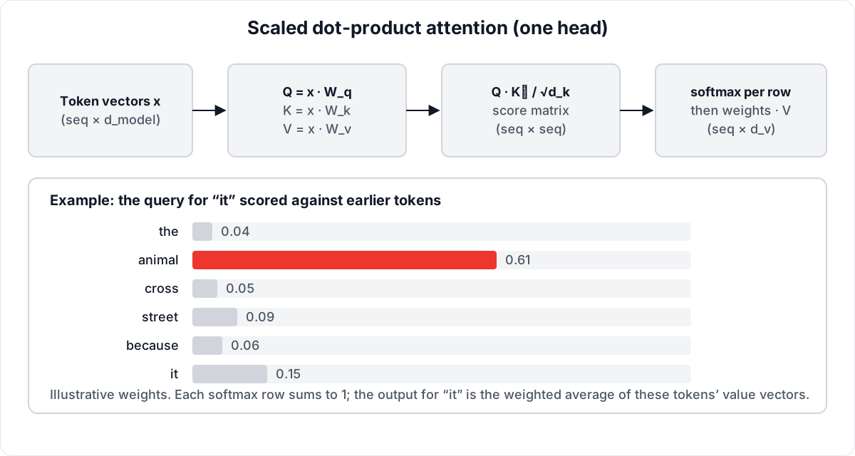
Attention end to end, with illustrative weights for the query of “it”. Diagram: Big Matrix Solutions, based on Attention Is All You Need.
Why causal masking matters
For a model predicting the next token, letting position 3 attend to position 7 would be cheating. It would see the answer during training.
The fix is a mask that sets scores for future positions to negative infinity before the softmax, which drives their weights to zero:
mask = torch.triu(torch.ones(seq, seq), diagonal=1).bool()
scores = scores.masked_fill(mask, float('-inf'))
This is the entire difference between an encoder (bidirectional, sees everything, good for classification) and a decoder (causal, sees only the past, good for generation). One triangular matrix.
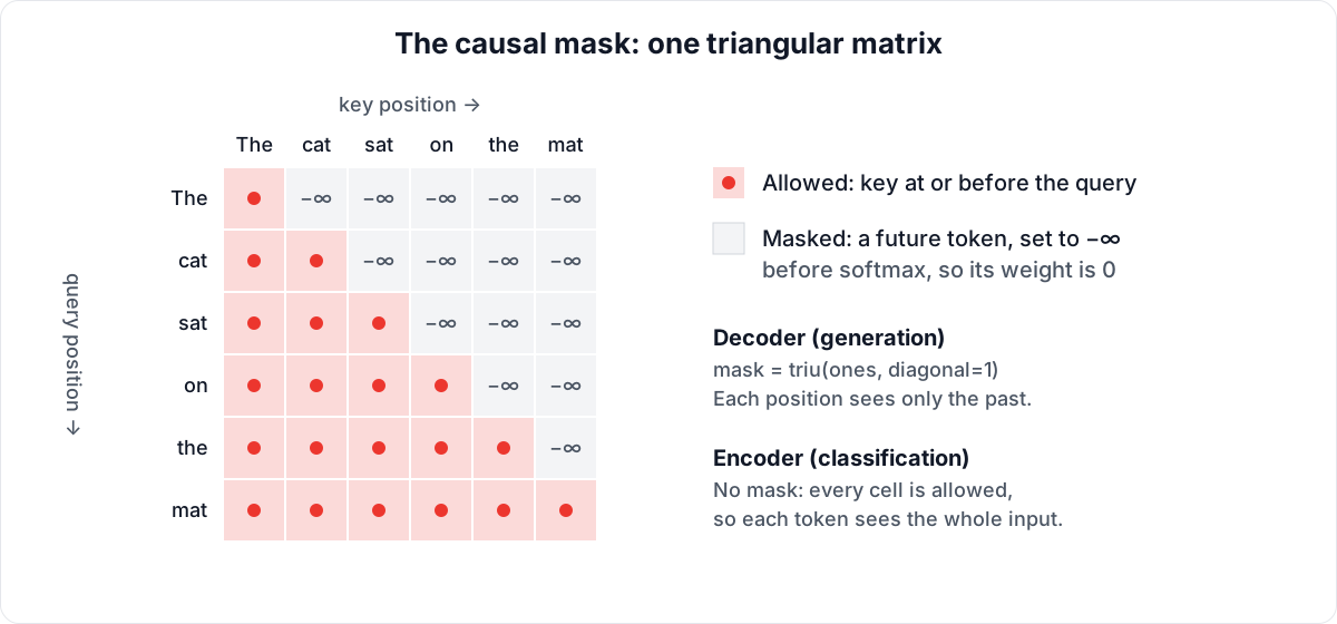
The causal mask: future positions are set to −∞ before the softmax. Diagram: Big Matrix Solutions, based on Attention Is All You Need.
Why multiple heads
One attention operation learns one notion of relevance. Language needs several at once: syntactic agreement, coreference, topical similarity, positional locality.
Multi-head attention runs several attention operations in parallel with separate projections, each in a lower-dimensional subspace, then concatenates the results:
# d_model = 768, n_heads = 12  ->  d_head = 64
# each head projects into 64 dims, attends, and the 12 outputs
# concatenate back to 768 and pass through W_o
The parameter count stays roughly the same as one big head, but you get twelve specialised relevance functions instead of one averaged one. Interpretability work has repeatedly found heads that specialise in strikingly legible ways: one tracking subject-verb agreement, another copying rare tokens from earlier in the context.
Step four: the feed-forward layer
After attention, each token passes independently through a two-layer MLP:
h = x @ W_1        # (d_model) -> (4 * d_model), e.g. 768 -> 3072
h = activation(h)  # GELU or SwiGLU in modern models
y = h @ W_2        # (4 * d_model) -> (d_model), 3072 -> 768
This looks like filler. It is not. This is where most of the parameters live, and it does a different job from attention.
The clean way to think about it: attention moves information between positions; the feed-forward layer processes information within a position.
Attention is a mixing operation. Without the MLP, stacking attention layers would just mix and re-mix the same vectors, and the whole stack would collapse to something close to linear. The MLP provides the nonlinear per-token computation: the actual thinking about what a token means, now that it has gathered its context.
There is also good evidence that these layers act as key-value memories, storing factual associations. Interpretability research has traced specific facts to specific feed-forward neurons and edited them. When you hear that a model "knows" something, the MLP layers are the most likely place it is stored.
The expansion to 4× width is not arbitrary. The wider intermediate layer gives room to compute many features before projecting back down, and 4× has proven a good empirical trade-off between capability and cost.
Step five: residuals and normalisation
The subtlest and most important part.
Each block is not x = attention(x). It is:
x = x + attention(norm(x))
x = x + feedforward(norm(x))
The x + is a residual connection, and it changes the semantics of the whole architecture.
Without residuals, each layer replaces its input. With them, each layer adds a correction to a running total. That running total is the residual stream, and it is the right mental model for a transformer: a wide channel carrying the token's representation from input to output, which each layer reads from and writes an update back into.
This buys three things:
- Gradients flow. The addition gives backpropagation a direct path from the loss to every layer, which is what makes 100-layer networks trainable at all.
- Layers can be gentle. A layer that finds nothing useful can contribute near-zero and leave the stream unharmed. It does not have to reconstruct its input.
- Composition works. Later layers read what earlier layers wrote. Circuits can span depth, with one layer establishing a feature and a later one using it.
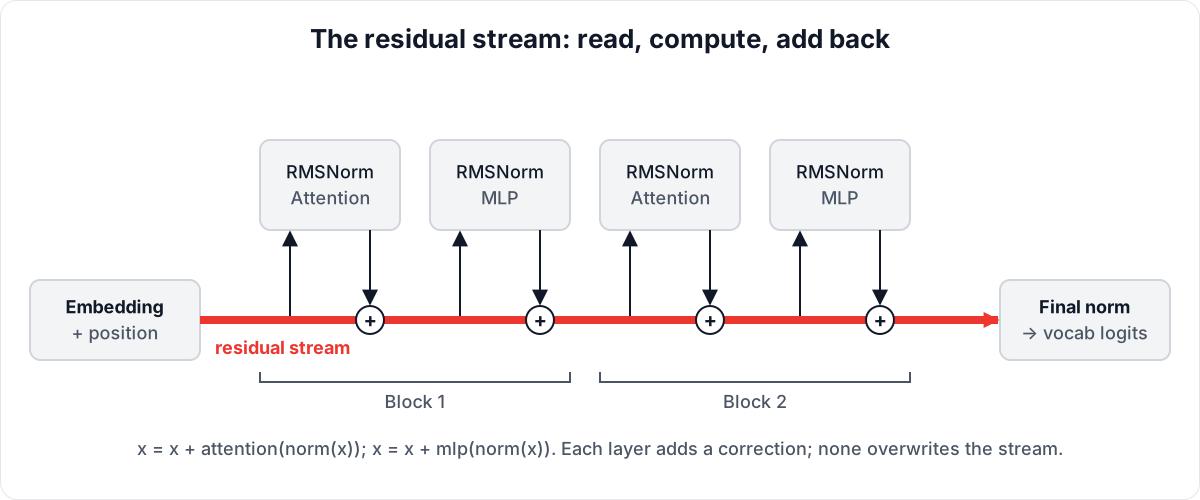
The residual stream: each sublayer reads through a norm and adds a correction back. Diagram: Big Matrix Solutions, based on Attention Is All You Need.
Layer normalisation stabilises activations to zero mean and unit variance across the feature dimension. Modern models use RMSNorm, a cheaper variant that skips mean-centring, and place it before the sublayer rather than after. Pre-norm is more stable at depth, which is why essentially every model since GPT-2 uses it.
Putting the stack together
class Block(nn.Module):
    def forward(self, x):
        x = x + self.attn(self.norm1(x))
        x = x + self.mlp(self.norm2(x))
        return x

class Transformer(nn.Module):
    def forward(self, ids):
        x = self.embedding(ids)
        for block in self.blocks:      # 12, 32, 80... layers
            x = block(x)
        x = self.final_norm(x)
        return self.output_head(x)     # -> vocab logits
That is the whole architecture. Embed, then repeat a block that mixes across positions and computes within them, then project to vocabulary logits.
The astonishing thing about transformers is not their complexity. It is that this much capability comes out of this little structure, repeated.
What each layer tends to do
Interpretability work has found a rough and reasonably consistent division of labour:
| Depth | Typical role |
|---|---|
| Early layers | Token identity, local syntax, surface patterns |
| Middle layers | Syntactic structure, entity tracking, factual recall |
| Late layers | Task-specific computation, output formatting, next-token prediction |
This is a tendency, not a rule, and it varies with training data and objective. But it is stable enough to be useful: if you are probing a model for factual knowledge, the middle layers are where to look.
The cost, and what it drives
Attention computes a score for every pair of tokens. That is O(n²) in sequence length, for both compute and memory.
At 1,000 tokens, a million scores per head per layer. At 100,000 tokens, ten billion. This quadratic term is the single reason long context is hard, and nearly every efficiency innovation of the last few years is an attack on it:
- FlashAttention: never materialises the full score matrix, computing it in tiles that fit in fast on-chip memory. Same mathematics, dramatically less memory traffic.
- Grouped-query attention: multiple query heads share one set of key and value heads, shrinking the KV cache that dominates memory during generation.
- Sliding-window attention: each token attends only to a nearby window, made global by stacking layers so information propagates across windows over depth.
- Sparse and linear attention: approximations that trade exactness for sub-quadratic scaling. Widely researched, less widely deployed at the frontier.
Notably, none of these change the core idea. The 2017 mechanism is intact; eight years of engineering has gone into computing it faster.
What to take away
If you keep four things:
Attention is learned, content-dependent routing. The score matrix decides which tokens inform which, and it is computed fresh from the content every time rather than fixed by architecture.
The residual stream is the real object. Layers read from and write to a shared channel. This is why circuits can span depth and why the architecture scales.
Attention mixes across positions; MLPs compute within them. You need both. Neither alone gets you anywhere.
Position is bolted on, and how you bolt it on matters. RoPE's relative-position geometry is a large part of why modern context windows are as long as they are.
Everything else (the exact activation, the norm placement, the head count, the width multiplier) is tuning. The four ideas above are the architecture.
Hero diagram: Transformer, full architecture by Daniel Voigt Godoy, CC BY 4.0, via Wikimedia Commons. Scaled and padded to fit; not otherwise altered.

Media credits:
- In-body diagrams (attention, causal mask, residual stream): Big Matrix Solutions, based on Attention Is All You Need (Vaswani et al., 2017).