
How Diffusion Models Work: Learning to Undo Noise, One Step at a Time
The elevator pitch for diffusion models is that they gradually turn noise into an image. True, and unhelpfully vague. It leaves out the part that makes the whole thing work, which is why breaking generation into many tiny steps makes an impossible problem tractable.
That is the idea worth understanding. Everything else follows from it.
Why generation is hard, and why steps help
Generating an image means sampling from a probability distribution over pixel arrays. For a 512×512 RGB image that is a distribution over roughly 786,000 dimensions, where an astronomically tiny fraction of the space contains anything that looks like a photograph.
Asking a network to jump from a random vector straight to a point in that tiny valid region is asking for a lot. GANs attempted it, and their notorious instability came largely from the difficulty of that single leap: a generator and discriminator locked in an adversarial game, with mode collapse and training divergence as constant companions.
Diffusion models make a different bargain. Instead of one enormous step, take a thousand small ones. Each step only has to remove a little noise, which is a vastly easier function to learn. And crucially, each step is trained with a plain regression loss: no adversary, no game, no instability.
You trade compute at generation time for tractability at training time. Given that training is done once and generation can be optimised afterwards, that turned out to be a very good trade.
Part one: the forward process (destroying an image)
The forward process is fixed, requires no learning, and is where the mathematics comes from.
Take a real image and add a small amount of Gaussian noise. Repeat, many times. After enough steps, nothing of the original remains. You have pure noise.
Formally, at each step t:
x_t = sqrt(1 - β_t) * x_{t-1} + sqrt(β_t) * ε where ε ~ N(0, I)
β_t is the noise schedule: how much noise to add at step t. It is small at first and grows, typically from around 1e-4 to 0.02 over 1,000 steps.
That definition is sequential, which would be painful for training. The convenient property of Gaussians is that you can jump to any step directly. Defining α_t = 1 - β_t and ᾱ_t as the cumulative product of all α up to t:
x_t = sqrt(ᾱ_t) * x_0 + sqrt(1 - ᾱ_t) * ε
One equation, any timestep, no loop. This is what makes training practical. Sample a random t, compute x_t in one shot, and train on it.
Note the structure: sqrt(ᾱ_t) scales down the original image while sqrt(1 - ᾱ_t) scales up the noise, and the two coefficients keep total variance roughly constant. At t = 0 you have the image. At t = T with ᾱ_T ≈ 0, you have pure noise. In between, a controlled blend.
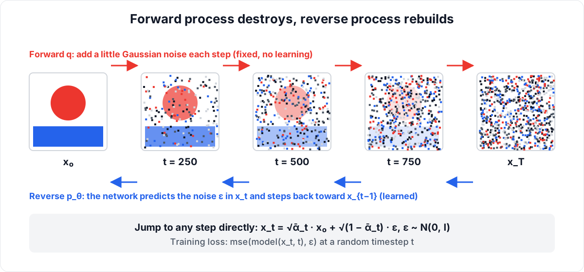
Forward noising is fixed; the reverse step is what the network learns. Diagram: Big Matrix Solutions, based on Denoising Diffusion Probabilistic Models.
Part two: the reverse process (learning to rebuild)
The forward process destroys. Generation needs the reverse: given x_t, produce x_{t-1}.
That reversal is not analytically available. It depends on the distribution of real images, which is exactly what we do not have in closed form. So we learn it with a neural network.
Here is the choice that trips people up. The network does not predict x_{t-1}. It does not predict x_0 either, in the standard formulation. It predicts the noise ε that was added.
# Training, in essence
t = random_timestep()
noise = torch.randn_like(x_0)
x_t = sqrt(alpha_bar[t]) * x_0 + sqrt(1 - alpha_bar[t]) * noise

predicted_noise = model(x_t, t)
loss = mse(predicted_noise, noise)
That is the entire training objective. Mean squared error between predicted and actual noise. No adversary, no complicated multi-term loss, no instability.
Why noise rather than the image? A few reasons that reinforce each other.
It falls out of the maths. Diffusion models derive from variational bounds on the data likelihood, and when you work through the algebra the tractable objective simplifies to noise prediction. The simple MSE loss is a reweighting of a principled bound.
The target has consistent scale. Noise is always unit Gaussian, at every timestep. Predicting x_0 from a very noisy input is a wildly harder task than from a nearly clean one, so an x_0-prediction target has enormously varying difficulty across t. Noise prediction is more uniform, which trains better.
It is equivalent anyway. Given x_t and a predicted ε, you can recover an estimate of x_0 by rearranging the forward equation. Nothing is lost.
Part three: sampling
At generation time you start from pure noise and step backwards.
x = torch.randn(shape)                     # pure noise

for t in reversed(range(T)):
    predicted_noise = model(x, t)

    # Estimate the clean image from the current state
    x_0_hat = (x - sqrt(1 - alpha_bar[t]) * predicted_noise) / sqrt(alpha_bar[t])

    # Take one step back toward t-1 (plus a little noise, except at the end)
    x = step(x_0_hat, x, t)

return x
Each iteration: look at the current noisy state, predict what noise is in it, use that to estimate the clean image, and move partway toward it. Then repeat.
The "partway" is important. If you jumped straight to x_0_hat you would get a blurry average, because early in the process the model genuinely cannot tell what the image is and its best estimate is a mean over many possibilities. Moving partway, then re-estimating, lets the sample commit gradually. Detail emerges over steps rather than being guessed at once.
Getting from 1,000 steps to 20
A thousand network evaluations per image is unusable in production. Two lines of work fixed this.
Better samplers. The reverse process can be viewed as an ordinary or stochastic differential equation, which means the whole numerical-integration literature applies. DDIM made the process deterministic and skippable, allowing 50 steps instead of 1,000. Higher-order solvers like DPM-Solver++ take larger, more accurate steps and produce good images in 20 to 30. The model is unchanged; only the integration is smarter.
Distillation. Train a student network to reproduce in one step what the teacher does in many. Progressive distillation halves step count repeatedly; consistency models and adversarial distillation push to one to four steps. There is a real quality cost at the extreme end, but for many uses that is a fair trade.
Part four: conditioning, which is what you actually want
Everything so far generates some image from the training distribution. Useful generation needs control.
Text conditioning works by feeding a text embedding into the denoiser, usually through cross-attention layers where image features attend to text tokens. The prediction becomes model(x_t, t, text). At every step, the noise estimate is shaped by the prompt.
But naive conditioning follows prompts weakly. The fix is classifier-free guidance, and it explains a slider you have almost certainly used.
During training, the text condition is randomly dropped some fraction of the time, so the same network learns both conditional and unconditional denoising. At sampling time you run both and extrapolate:
eps_cond   = model(x_t, t, prompt)
eps_uncond = model(x_t, t, None)

eps = eps_uncond + guidance_scale * (eps_cond - eps_uncond)
The difference (eps_cond - eps_uncond) is the direction the prompt pulls in. Multiplying it by a scale greater than one exaggerates that pull, pushing the sample further toward the prompt than the model's honest conditional estimate would.
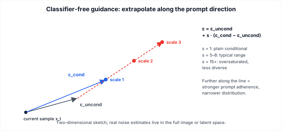
Classifier-free guidance pushes past the conditional estimate along the prompt direction. Diagram: Big Matrix Solutions, based on Classifier-Free Diffusion Guidance.
This is exactly the CFG scale in every image tool:
| Scale | Behaviour |
|---|---|
| 1.0 | No guidance; loose prompt adherence, high diversity |
| 5–8 | Typical range; good balance |
| 15+ | Strong adherence, oversaturated, reduced diversity |
The trade-off is fundamental rather than a tuning artefact. Guidance improves prompt fidelity by narrowing the distribution you are sampling from, and a narrower distribution is by definition less diverse. There is no setting that gives you both.
Part five: latent diffusion
One more piece, and it is the one that made this technology widely deployable.
Running diffusion in pixel space is expensive. A 512×512 image is 786,000 dimensions, and you are evaluating a large network on it dozens of times per sample.
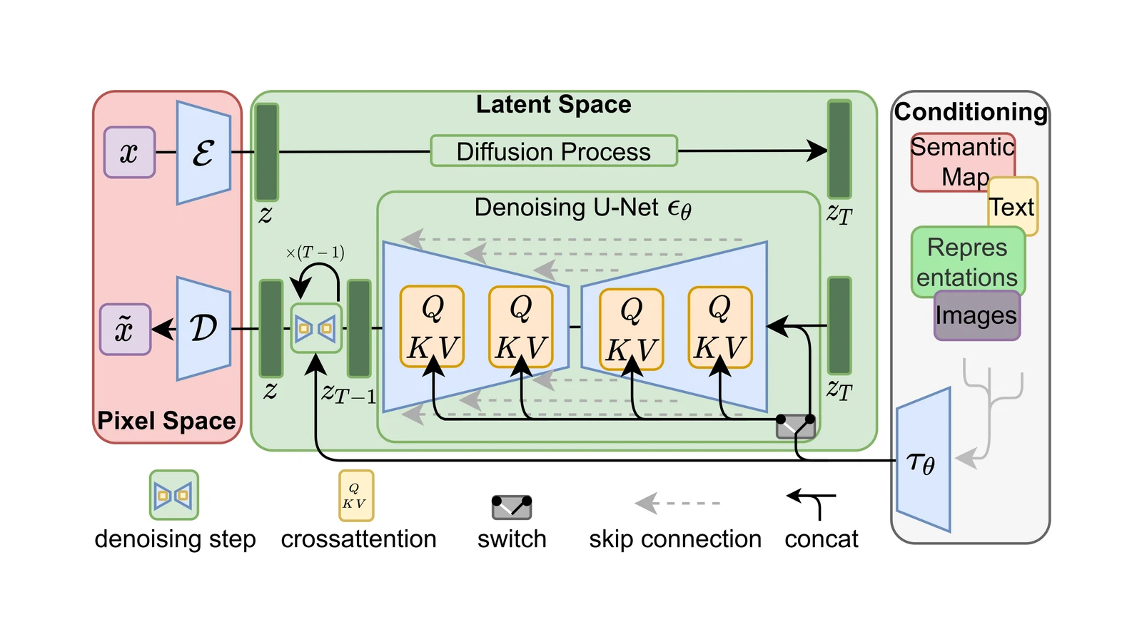
Latent diffusion moves the process into a compressed space:
- Train an autoencoder that compresses images roughly 8× per spatial dimension, taking 512×512×3 down to 64×64×4.
- Run the entire diffusion process in that latent space.
- Decode the final latent back to pixels once.
The compression is about 48× in element count, and the compute saving is comparable. Critically, the autoencoder is trained to preserve perceptual content, so the discarded information is largely imperceptible detail rather than structure.
This is why Stable Diffusion could run on consumer hardware, and every practical image system since has used the same trick.
The denoiser itself
What network predicts the noise? Historically, a U-Net, and the fit is not a coincidence.
The task needs global understanding (what is this image of, so denoising is coherent) and pixel-precise output (noise is per-pixel). That is precisely the semantics-plus-localisation tension U-Net was designed for, and its skip connections route high-resolution detail around the bottleneck.
The diffusion version adds:
- Timestep embedding: the network must know the noise level, since the right behaviour at t=900 differs completely from t=50. Injected as a sinusoidal or learned embedding into every block.
- Self-attention at lower resolutions: for global coherence, applied where spatial dimensions are small enough for quadratic attention to be affordable.
- Cross-attention: where text conditioning enters.
At the largest scales, pure transformer denoisers (diffusion transformers) have overtaken U-Nets, scaling more predictably with parameters and data. Below that scale the U-Net remains extremely competitive and is what most systems run.
What actually matters in practice
If you are working with these models rather than building them:
Steps have diminishing returns fast. With a modern sampler, 20 to 30 steps is usually indistinguishable from 100. Going to 150 mostly burns compute. Test on your own prompts and find where your curve flattens.
Guidance scale is a diversity dial as much as a quality dial. If outputs feel repetitive and overcooked, lower it. If prompts are being ignored, raise it. If both are wrong, the problem is the prompt or the model, not the scale.
The negative prompt is not magic. It replaces the unconditional branch of CFG with a conditional one on the negative text, so you are extrapolating away from that description. It works because of the same subtraction, which also means an overloaded negative prompt pulls in incoherent directions.
Seeds are fully deterministic with deterministic samplers. Same seed, same prompt, same settings, same sampler gives the same image. This is genuinely useful for iterating on a prompt while holding composition roughly fixed.
Why diffusion won
For a few years, GANs were the state of the art in image generation and diffusion was a curiosity. The reversal came down to three things.
Stable training. An MSE regression loss is about as well-behaved as objectives get. No adversarial dynamics, no mode collapse, no discriminator balance to babysit.
Mode coverage. GANs are prone to dropping parts of the data distribution entirely. Diffusion models, trained to model the whole thing through a likelihood-derived objective, cover it far more completely.
Clean scaling and conditioning. Bigger models and more data reliably help, and classifier-free guidance gave a principled control mechanism that GAN conditioning never matched.
The compute cost at inference was the one real disadvantage, and better samplers plus latent-space operation plus distillation reduced it by two orders of magnitude.
Which is a fairly common pattern in this field: the method that wins is not the one that was fastest at the start, but the one whose main problem turned out to be an engineering problem.
Hero diagram: latent diffusion architecture by Rombach, Blattmann, Lorenz, Esser and Ommer, CC BY 4.0, via Wikimedia Commons. Scaled and padded to fit; not otherwise altered.

Media credits:
- In-body diagrams (forward/reverse process, classifier-free guidance): Big Matrix Solutions, based on Ho et al., 2020 and Ho and Salimans, 2022.